I tend to be highly critical of political commentators, and it is not uncommon for me to get them in my recommended section on YouTube. One of the aspects that intrigues me is the use of advanced rhetoric to appeal to large masses of people, usually through founding their arguments on ideological stands. This drove to develop a way to use sentiment analysis to explore relationships that might the success of such strategy. I was able to achieve this by fetching data from APIs, including the captions from subtitles, and stats from the videos. In these chunks of code, I chose Ben Shapiro as a subject of study.
Libraries and functions
library(tidyverse)
library(reticulate)
library(rvest)
library(jsonlite)
library(olsrr)

getwordcloud = function(c){
  library(tm)
  library(syuzhet)
  load("/Users/jevz/Downloads/sysdata.rda")
  str = subs[k %in% c] %>%
    str_split('\\s') %>% unlist %>%
    str_subset('\\w+') %>%
    str_extract('\\w+') %>%
    str_remove_all('\\s') %>%
    unlist %>%
    table %>%
    sort
  str.n = str %>% names()

  v = (str[str.n %in% syuzhet_dict$word] %>% unname %>% unlist)
  w = str.n[str.n %in% syuzhet_dict$word]
  cloud = data.frame(v,w) %>% tail(n = 100)

  wordcloud::wordcloud( cloud$w,cloud$Freq)

  # subs[1]
  # subs[k %in% 2] %>%
  #   str_split('\\s') %>%
  #   str_subset('\\w+') %>%
  #   unlist %>% table %>%
  #   sort %>% head(n = 10)
}

new.rollmean = function(vec, target){
  if(length(vec)<target){
    ret = vec
  }
  else{
    ret = zoo::rollmean(vec, length(vec) - target + 1) %>%
      na.omit()
  }
  return(ret)
}

youtube= function(id){
  rq = import(module = 'requests', as = 'rq',convert = T)
  url = "https://youtube-v31.p.rapidapi.com/videos"

  querystring = list("part"="contentDetails,snippet,statistics","id"= id)

  headers = list(
    'x-rapidapi-host'= "youtube-v31.p.rapidapi.com",
    'x-rapidapi-key'= ""
  )

  response = rq$request("GET", url, headers=headers, params=querystring)$text

  ret = response %>% fromJSON()
  ret = ret$items
  ret1 = ret$snippet
  ret2 = ret$statistics


  # return(list(
  #   snippet = ret1,
  #   stats = ret2,
  #   join = ret1[1:3] %>% cbind(ret2) ))
  return(
    ret2 %>% as.numeric())
}

lu.sub = function(query){
  rq = import('requests')
  # sample query = "I'm beginnin' to feel like a Rap God"
  url = "https://subtitles-for-youtube.p.rapidapi.com/subtitles/searchInSubtitles"

  querystring = list("query"=query)

  headers = list(
    'x-rapidapi-host'=  "subtitles-for-youtube.p.rapidapi.com",
    'x-rapidapi-key' = ""
  )

  response = rq$request("GET", url, headers=headers, params=querystring)

  return(
    (response$text %>% jsonlite::fromJSON())$videos
  )
}

get.sub = function(ID){
  rq = import('requests')

  url = paste0("https://subtitles-for-youtube.p.rapidapi.com/subtitles/",ID)

  headers = list(
    'x-rapidapi-host'= "subtitles-for-youtube.p.rapidapi.com",
    'x-rapidapi-key'= ""
  )

  response = rq$request("GET", url, headers=headers)

  captions = response$text %>% jsonlite::fromJSON()
  ret = captions$text %>% paste(collapse = ' ')
  return(ret)}

channel.vid = function(ID){
  rq = import('requests')
  url = "https://youtube-v31.p.rapidapi.com/search"
  querystring = list("channelId"=ID,
                     "part"="snippet,id",
                     "order"="date","maxResults"="50")

  headers = list(
    'x-rapidapi-host'= "youtube-v31.p.rapidapi.com",
    'x-rapidapi-key'= ""
  )

  response = rq$request("GET", url, headers=headers, params=querystring)
  return(response$text %>% jsonlite::fromJSON())
}

get.channelId=function(url){(read_html(url) %>%
                               html_nodes('*') %>%
                               html_text() %>%
                               str_split('\\n') %>% unlist %>%
                               str_subset('"externalId":') %>%
                               str_extract_all('externalId.+keyw') %>%
                               str_extract(':.+,') %>%
                               str_remove_all('^..|.,') )[1]}

countwords = function(str1){
  lengths(gregexpr("\\W+", str1)) + 1
}

find.titles = function(c){
  res = cbind( data[k %in% c,], videoId = data[ k %in% c ,] %>% rownames %>% as.factor )
  mat$videoId = mat$videoId %>% as.factor()
  res = mat %>% inner_join(res)
  res$title}
Extracting and wrangling data
url = 'https://www.youtube.com/channel/UCnQC_G5Xsjhp9fEJKuIcrSw'
df = channel.vid(get.channelId(url))

tb = df$items$snippet %>% as.data.frame()
tb2 = df$items$id %>% as.data.frame()
mat = cbind(
  (tb2 %>% select(videoId,kind)),
  tb %>%
    select(publishedAt,title,description,)
) %>% filter(kind == 'youtube#video') %>% select(-kind)
str = mat$videoId %>% head(n = 30)
stats = sapply(str, youtube) %>% t
colnames(stats) =  c("viewCount",     "likeCount", "favoriteCount",  "commentCount")
subs = sapply(str,get.sub)
count = sapply(subs, countwords)
data = syuzhet::get_nrc_sentiment(subs) %>% cbind(stats)

for( i in 1:length(count)){
  data[i,1:10] = (data[i,1:10]/count[i])*mean(count)
}

emotions = data.frame(
  (data[,1:10] %>% colSums),(data[,1:10] %>% colnames())
)

lm.data = data.frame(likes = data$likeCount, data[,1:10])
colnames(lm.data) = colnames(lm.data) %>% toupper()

lm.data2 = c()
for(i in 1:8){
  entry = cbind(emotion = data[,i], likes = data$likeCount, name = colnames(data)[i])
  lm.data2 = rbind(lm.data2,entry )
}
lm.data2 = lm.data2 %>% as.data.frame()
lm.data2[,3] = lm.data2[,3] %>% as.factor()
lm.data2[,1] = lm.data2[,1] %>% as.numeric()
lm.data2[,2] = lm.data2[,2] %>% as.numeric()

k = kmeans(data[,1:8],3)[[1]]
pca = cbind(prcomp( data[,1:8] %>% as.matrix, scale=TRUE)$x, k) %>% as.data.frame()
pca$k = pca$k %>% as.factor()

datac = cbind(data,k = k %>% as.factor())
Emotions in all videos
Just a quick summary of how many words assosiated with each emotion are present in all of the videos (n = 30).
ggplot(emotions) +
  aes(
    x = X.data...1.10......colnames...,
    fill = X.data...1.10......colnames...,
    weight = X.data...1.10......colSums.
  ) +
  geom_bar() +
  scale_fill_hue(direction = 1) +
  theme_minimal() +
  labs(title = ('Distribution of emotions across all videos'))+
  xlab('Emotions')+ylab('Freq')+
  theme(legend.position = "none")

Likes and sentiments
Before looking a bit more into the emotions, we can also see how each sentiment (positive and negative) is assosiated with the amount of likes the video got/
ggplot(data) +
  geom_point(mapping = aes(x = positive, y = likeCount),
             size = 2, colour = "steelblue") +
  geom_smooth(mapping = aes(x = positive, y = likeCount),method ='lm', alpha = 0,linetype = 5,
              size = .75, colour = "steelblue") +
  geom_point(mapping = aes(x = negative, y = likeCount),
             size = 2, colour = "darkred") +
  geom_smooth(mapping = aes(x = negative, y = likeCount),,method ='lm', alpha = 0, linetype = 5,
              size = .75, colour = "darkred") +
  xlab('Sentiment')+
  ylab('Likes')+
  labs(title = ('Likes by sentiment'),
       subtitle = 'Positive sentiments shown as blue and negative as red')+
  theme_minimal()
## `geom_smooth()` using formula 'y ~ x'
## `geom_smooth()` using formula 'y ~ x'

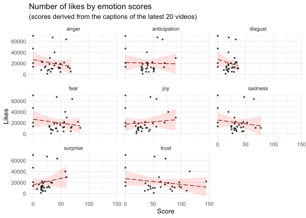
Linear model
We can do the same with the 8 emotions being studied, where through linear models we can fit a trend line for each of the variables.
lm = lm(LIKES ~., lm.data)
# stargazer::stargazer(lm,type = 'text')

# fit.info = olsrr::ols_step_all_possible(model = lm)
# fit.info[fit.info$rsquare %>% which.max(),]

lm2 = lm(likes ~.*.,lm.data2)

ggeffects::ggpredict(
  lm2,
  terms = c('emotion', 'name')
) %>% plot(alpha = 0)

# lm2 %>% stargazer::stargazer(type = 'html')

ggplot(data = lm.data2, aes(emotion, likes), color = name) +
  geom_smooth(color = 'darkred', method = 'lm', size = .5, alpha = .15, linetype = 5, fill = 'red') +
  geom_point(color = 1, size = .75, alpha = .75) +
  labs(title = "Number of likes by emotion scores",
       subtitle = "(scores derived from the captions of the latest 20 videos)",
       y = "Likes", x = "Score") +
  facet_wrap(~ name) + theme_minimal()
## `geom_smooth()` using formula 'y ~ x'
Unsupervised clustering by k-means
We can also start messing with a bit of machine learning and get to cluster our data based on the emotions. This can best be seen in the PCA plot below.
a = ggplot( data = pca, aes(PC1,PC2, colour = k))+
  geom_jitter(size = 4, width = 1, alpha = .7) + theme_minimal()+
  labs(title = 'Principal compenent analysis')

b = ggplot(datac) +
  aes(x = likeCount, fill = k, colour = k) +
  geom_histogram( bins = 10, alpha = .75) +
  xlab('Likes')+ylab('Freq')+labs(title = "Distribution of likes",
                                  subtitle = 'grouped by kmeans')+
  theme_minimal()
gridExtra::grid.arrange(a,b)

Word clouds by k-mean groups
For each of the k-means clusters, we can also fetch the titles of the videos and start looking at what were the most frequent wordfs through a word cloud.
We can also start trying to interpret how each of the clusters were formed by looking for patterns in the video titles of each group.
try({
  par(mar= rep(0,4))
  find.titles(1) %>% print
  getwordcloud(1)
})
##  [1] "Shapiro Breaks Down CDC Director's SHOCKING Covid Admission"
##  [2] "Democrats to Allow NON-CITIZENS to Vote in NYC"
##  [3] "Shapiro RIPS Biden's Jan. 6th Speech"
##  [4] "Biden Explains Why He Didn't Use Trump's Name During Jan. 6th Speech"
##  [5] "INSANE: Jail Time Will No Longer Be Given for THESE Crimes in NYC..."
##  [6] "New York Times Op-Ed Makes ABSURD Claim — Shapiro Reacts"
##  [7] "Comedian Patton Oswalt Apologizes For Posting Picture With Dave Chappelle"
##  [8] "Unhinged TikToker Gives Police Officers "Pig Bait""
##  [9] "LOL: Australian TikToker Has No Idea What She's Talking About"
## [10] "The Infinite Woke TikTok Loop of Stupidity"
## [11] "Ben Shapiro Breaks Down the Top Mainstream Media Fails of 2021"
## [12] "LOL: Demi Lovato Sings to Ghost to Help It Overcome Trauma"

try({
  par(mar= rep(0,4))
  find.titles(2) %>% print
  getwordcloud(2)
})
##  [1] "Justice Sotomayor Proves That She Is Not Wise | Ep. 1408"
##  [2] "Ben Shapiro REACTS to Insane Woke TikToks | Volume 6"
##  [3] "It’s The Democrats’ January 6 Spectacular!!! | Ep. 1407"
##  [4] "Democrats MELT DOWN Over January 6th Anniversary — Kamala Compares Jan 6th to 9/11"
##  [5] "The Democrats' January 6th Push To Ruin Democracy | Ep. 1406"
##  [6] "Ben Shapiro Reviews the 'Yellowstone' Season 4 Finale!"
##  [7] "California Mandates GENDER-NEUTRAL Toy Sections"
##  [8] "You Aren’t The Only Person In The World | Ep. 1405"
##  [9] "The Exploitation Of January 6 | Ep. 1404"
## [10] "Happy New Year, Everyone Is Still Stupid | Ep. 1403"
## [11] "New York Magazine Features Transgender Man on Cover"
## [12] "The Penis Mightier Than The Sword | Ep. 1401"
## [13] "Infinity Days To Stop The Spread | Ep. 1400"
## [14] "Jordan Peterson on the Consequences of Free Speech"

try({
  par(mar= rep(0,4))
  find.titles(3) %>% print
  getwordcloud(3)
})
## [1] "LOL: AOC's HYPOCRISY on Full Display in Florida"
## [2] "Satanist TikToker Identifies as a NIGHTMARE"
## [3] "Leftists Wanted to HOLD VACCINE Until After Trump's Presidency"
## [4] "Jordan Peterson Gives the Best Relationship Advice You’ll Ever Hear"
## Error in -freq : invalid argument to unary operator
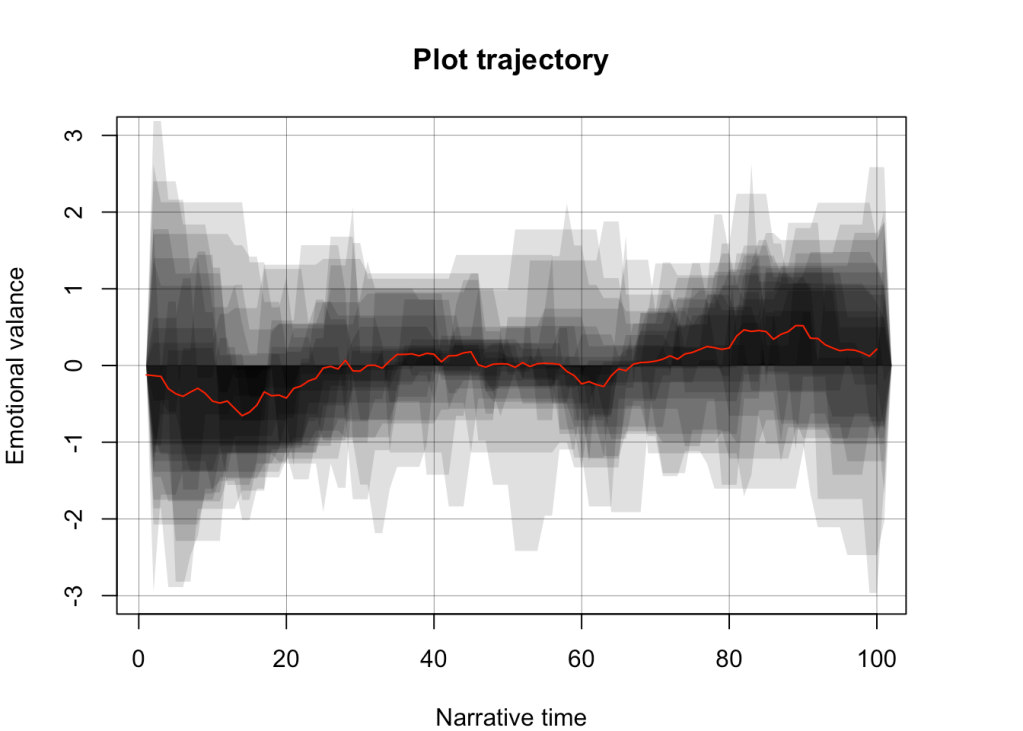
Emotional valance in the plot trajectory
I finallize my curiosity by plotting how the emotional valance of each video changes as time progresses we do this by both scaling the time frames (throgh rolling means) and the actual valance score.
I interpret the cosine looking wave as a proper communication strategy, where the commenter gives a ride to the listener through negative and positive charged words.
par(mar= rep(4,4))
plot(NULL,
     xlim = c(1,100),
     ylim = c(-3,3),
     xlab = 'Narrative time',
     ylab = 'Emotional valance',
     main = 'Plot trajectory')
grid(lwd = .25, lty = 7, col = 1)

list = c()
for( i in 1:length(subs[count>10]) ){
  poa_word_v <- get_tokens(
    subs[count>10][i],
    pattern = "\\W")

  narr = get_sentiment(
    poa_word_v,
    method="syuzhet"
  )

  entry = (new.rollmean(vec = narr, target = 100)) %>% scale

  c(0, entry, 0) %>%
    polygon(col = 1 %>% alpha(.15), border = NA)
  list = rbind(list,matrix((new.rollmean(vec = narr, target = 100)) %>% scale, nrow = 1))
}
list  %>% colMeans() %>% lines(col = "red")