
In order to interpret the content of the posts in the ‘trending’ section, we will be using a webdriver that fetches the text and run it through the NRC Emotion Lexicon sentiment analysis. Some interesting findings were how the news section seemed to be filled with more sentiment-loaded words relative to the rest of the posts, that posts which included joyful words were likely to have more likes, and that even though posts that included fearful words were more likely to receive less likes although it was the most prevalent.
A tidier copy of the documentation can be found at https://emiliovel-gettr.netlify.app
The NRC Emotion Lexicon is a list of English words and their associations with eight basic emotions (anger, fear, anticipation, trust, surprise, sadness, joy, and disgust) and two sentiments (negative and positive).
Libraries, functions, and web-driver set up
We load all the needed packages.
We also define some functions we will be needing. One of them to find the maximum values of a vector, allowing for multiple matches. Meanwhile, the other functions simply counts how many words are in a given vector
Finally, we just set up a selenium web-driver in our computer. Even though we are not really doing web-crawling, it is important we use RSelenium to get the source html since alternative methods like read_html() will not work.
library(rvest)
library(tidyverse)
library(RSelenium)
library(syuzhet)
library(stargazer)

mx = function(myVector){
  which( myVector == max(myVector) )
}

countwords = function(str1){
  lengths(gregexpr("\\W+", str1)) + 1
}

url = 'https://www.gettr.com/trending'

rD = rsDriver(browser = "firefox",
              port = 4252L,
              verbose = F)
remDr = rD$client
Webscrapping and data-wrangling
The code used to scrap and wrangle the data. It includes some very lose inline commentary.
## get the html source
remDr$navigate(url)
Sys.sleep(1)
for(i in 1:5){
  webElem = remDr$findElement("css", "body")
  webElem$sendKeysToElement(list(key = 'end' ))#scroll down
  Sys.sleep(.75)
  # print(i)
}
src = remDr$getPageSource()[[1]]

classes = src %>%
  read_html %>%
  html_nodes("*") %>%
  html_attr("class") %>%
  unique %>%
  str_subset('timeline') %>%
  str_replace_all('\\s', '.')

## Fetch the posts and relevant info
posts = c()
for (i in 1:length(classes)) {
  post = src %>%
    read_html %>%
    html_nodes(paste0('div.', classes[i])) %>%
    html_text()
  posts = c(posts, post)
}

dates = posts %>%
  str_subset('\\n') %>%
  str_extract('·\\w+\\s\\d{1,2},\\s\\d{4}') %>%
  str_remove_all('·')

comments = posts %>%
  str_subset('\\n') %>%
  str_extract('\\d{1,100}Like') %>%
  str_remove_all('Like')

likes = posts %>%
  str_subset('\\n') %>%
  str_extract('Like.+Repost') %>%
  str_remove_all('Like|Repost')

likes[grepl('K', likes)] = (likes[grepl('K', likes)] %>% parse_number()) *
  1000
likes = likes %>% parse_number()

shares = posts %>%
  str_subset('\\n') %>%
  str_extract('Repost.+Share') %>%
  str_remove_all('Share|Repost')

nrc = c()

for (i in 1:((posts %>% str_subset('\\n')) %>% length)) {
  senti = ((posts %>%
              str_subset('\\n'))[i]) %>%
    str_remove_all(paste0('\\s', tm::stopwords(), '\\s', collapse = '|')) %>%
    str_extract('\\n.+') %>%
    str_remove_all('\\n') %>%
    str_split('\\s') %>%
    unlist %>%
    get_nrc_sentiment() %>%
    colSums()
  senti = c(senti, total = senti %>% sum)

  nrc = rbind(nrc, senti)
}

df = data.frame(dates, comments, likes, shares, nrc)
rownames(df) = NULL

## Fetch the most mentioned websites
websites = posts %>%
  str_extract('www\\S+com') %>%
  na.omit() %>%
  table %>%
  sort %>% as.data.frame()

## Fetch the news sidebar section
news.senti = src %>%
  read_html() %>%
  html_nodes('div.sidebar-body') %>%
  html_text() %>%
  str_extract_all('\\w+') %>%
  unlist %>%
  get_nrc_sentiment()

lbs = nrc[,1:10] %>% colnames()
posts.news = rbind.data.frame(
  cbind((nrc[,1:10] %>% colSums)/nrow(nrc), 'Posts',lbs ),
  cbind((news.senti %>% colSums)/nrow(nrc), 'News',lbs ))
posts.news[,1] = posts.news[,1] %>% as.numeric()
posts.news[,2] = posts.news[,2] %>% as.factor()
posts.news[,3] = posts.news[,3] %>% as.factor()

## Wrangle the data for a (probably faulty) lm
lm.data2 = c()
for (i in 1:10){
  entry = cbind(likes,nrc[,i], colnames(nrc)[i])
  lm.data2 = rbind(lm.data2, entry)
}
lm.data2 = data.frame(lm.data2)
colnames(lm.data2) = c('Likes','Score','Emotion')
lm.data2[,1] = lm.data2[,1] %>% as.numeric()
lm.data2[,2] = lm.data2[,2] %>% as.numeric()
lm.data2 = lm.data2 %>%
  filter(Emotion != 'positive') %>%
  filter(Emotion!='negative')
lm.data2[,3] = lm.data2[,3] %>% as.factor()

lm2 = lm(Likes ~ .*., lm.data2)

##  Get the overall frequency of sentiments
overall.freq =  data.frame(colSums(nrc[, 1:10]), colSums(nrc[, 1:10]) %>% names)

## Wrangle the data for a (better) lm; this includes looking for the predominant sentiment(s) in each post
lm.data = data.frame(l = df$likes, nrc)
for (i in 2:ncol(lm.data)){
  lm.data[,i] = lm.data[,i] %>% scales::rescale()
}

factors = c()
for (i in 1:length(apply(lm.data[,2:11], 1, mx))){
  factors = c( factors, apply(lm.data[,2:11], 1, mx)[[i]] %>% names %>% str_extract_all('^\\w{1,3}|\\s\\w{1,3}') %>% paste(collapse = '-') )
}

lm.data = data.frame(likes = df$likes,
                     Sentiments = factors
)[(sapply(factors, countwords)<5),]
lm.data[,2] = lm.data[,2] %>% as.factor()
lm = lm(likes ~ .*., lm.data)

## Look for the frq of the predominant sentiment(s)
complex.sent = data.frame(
  table(lm.data[,2]) %>% sort,table(lm.data[,2]) %>% sort %>% names
)

rD$server$stop()
Most mentioned websites
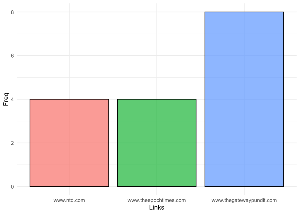
We can fetch and visualize the frequency of the links mentioned in posts in GETTR.
I find it interesting that out of 16 links, there are only 3 different “sources”, which I would interpret as a a site with a very centralized media.
ggplot(websites) +
  aes(x = ., fill = ., weight = Freq) +
  geom_bar(alpha = .75, col = 1) +
  scale_fill_hue(direction = 1) +
  labs(x = "Links", y = "Freq") +
  theme_minimal() +
  theme(legend.position = "none")
websites %>% head %>% knitr::kable()
Posts & News
We can look and contrast at the sentiment scores for each section of the site, the posts and the news in the sidebar section.
The graphical results are very interesting. After having both section’s sentiments scaled, we can see that that both sections follow a similar distribution of scores, although, the news section’s scores seem to be amplified.
I would interpret this as that the news provider most likely folllow a strategy that involves using highly emotional words in order to grab the reader’s attention.
ggplot(posts.news) +
  aes(x = lbs, fill = V2, weight = V1) +
  geom_bar(alpha = .75, col = 1) +
  scale_fill_hue(direction = 1) +
  labs(x = "Sentiments", y = "Scores") +
  theme_minimal()

posts.news %>% head %>% knitr::kable()
| V1 | V2 | lbs | |
|---|---|---|---|
| anger | 0.1428571 | Posts | anger |
| anticipation | 1.4285714 | Posts | anticipation |
| disgust | 0.1428571 | Posts | disgust |
| fear | 0.4761905 | Posts | fear |
| joy | 0.7619048 | Posts | joy |
| sadness | 0.1428571 | Posts | sadness |
Likes and scores
We can also start looking at the relationship between likes and different scores. As a first attempt, we can try to look at the relationship of each of the sentiments and the number of likes, regardless of the combination of other emotions.
After testing the linear model, we see that there is no significant relationship between the variables (probably caused by the odd way the data is structured). Either way this allows us to fit trend lines across our scatter plot.
ggplot(lm.data2) +
  aes(x = Score, y = Likes, colour = Emotion) +
  geom_jitter(shape = "circle", size = 2, width = .2, alpha = .75 ) +
  scale_color_hue(direction = 1) +
  theme_minimal()

lm2 = lm(Likes ~ .*., lm.data2)
ggeffects::ggpredict(lm2,
                     c('Score','Emotion'),
                     ci = F
) %>% plot

lm.data2 %>% head %>% knitr::kable()
| Likes | Score | Emotion | |
|---|---|---|---|
| senti | 1300 | 0 | anger |
| senti.1 | 957 | 0 | anger |
| senti.2 | 242 | 0 | anger |
| senti.3 | 374 | 0 | anger |
| senti.4 | 143 | 0 | anger |
| senti.5 | 440 | 0 | anger |
stargazer(lm2, type = 'html')
| Dependent variable: | |
| Likes | |
| Score | -334.722 |
| (393.910) | |
| Emotionanticipation | -51.314 |
| (289.315) | |
| Emotiondisgust | 0.000 |
| (210.554) | |
| Emotionfear | 153.830 |
| (231.660) | |
| Emotionjoy | -168.747 |
| (266.129) | |
| Emotionsadness | -8.278 |
| (210.554) | |
| Emotionsurprise | -30.617 |
| (207.765) | |
| Emotiontrust | -15.962 |
| (251.315) | |
| Score:Emotionanticipation | 337.170 |
| (419.534) | |
| Score:Emotiondisgust | -0.000 |
| (557.074) | |
| Score:Emotionfear | -88.738 |
| (458.574) | |
| Score:Emotionjoy | 493.442 |
| (454.155) | |
| Score:Emotionsadness | 57.944 |
| (557.074) | |
| Score:Emotionsurprise | 154.117 |
| (612.914) | |
| Score:Emotiontrust | 308.993 |
| (411.720) | |
| Constant | 655.722*** |
| (148.884) | |
| Observations | 168 |
| R2 | 0.037 |
| Adjusted R2 | -0.058 |
| Residual Std. Error | 631.662 (df = 152) |
| F Statistic | 0.392 (df = 15; 152) |
| Note: | p<0.1; p<0.05; p<0.01 |
Looking at the overall sentiments
Before moving forward and upgrading our linear model, we can still look at the overall score of sentiment analysis in the posts. We can do this by just consider at the aggregate scores.
ggplot(overall.freq) +
  aes(
    x = colSums.nrc...1.10.......names,
    fill = colSums.nrc...1.10.......names,
    weight = colSums.nrc...1.10..
  ) +
  geom_bar(alpha = .75, col = 1) +
  scale_fill_hue(direction = 1) +
  labs(x = "Sentiments", y = "Freq") +
  theme_minimal() +
  theme(legend.position = "none")

overall.freq %>% head %>% knitr::kable()
| colSums.nrc…1.10.. | colSums.nrc…1.10…….names | |
|---|---|---|
| anger | 3 | anger |
| anticipation | 30 | anticipation |
| disgust | 3 | disgust |
| fear | 10 | fear |
| joy | 16 | joy |
| sadness | 3 | sadness |
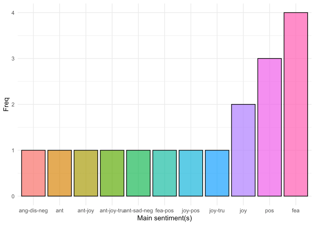
Predominant sentiment(s)
In order to upgrade our model, we can redesign the data and focus on the predominant sentiment for each post, while allowing for more complex sentiments given the case there is a ‘tie’ between scores. Ultimately we can just repeat the step from the last chunk and look at the aggregate score of our re-defined sentiments. In order to be able to visualize our data through ggeffects, we also drop predominant sentiments that are made up from 5 or more words.
Note: Due to having our renamed sentiments have long names, I have abbreviated them by just keeping the first three letter of each emotion.
ggplot(complex.sent) +
  aes(x = Var1, fill = Var1, weight = Freq) +
  geom_bar(alpha = .75, col = 1) +
  scale_fill_hue(direction = 1) +
  labs(x = "Main sentiment(s)", y = "Freq") +
  theme_minimal() +
  theme(legend.position = "none")
complex.sent %>% head %>% knitr::kable()
| Var1 | Freq | table.lm.data…2…….sort…..names |
|---|---|---|
| ang-dis-neg | 1 | ang-dis-neg |
| ant | 1 | ant |
| ant-joy | 1 | ant-joy |
| ant-joy-tru | 1 | ant-joy-tru |
| ant-sad-neg | 1 | ant-sad-neg |
| fea-pos | 1 | fea-pos |
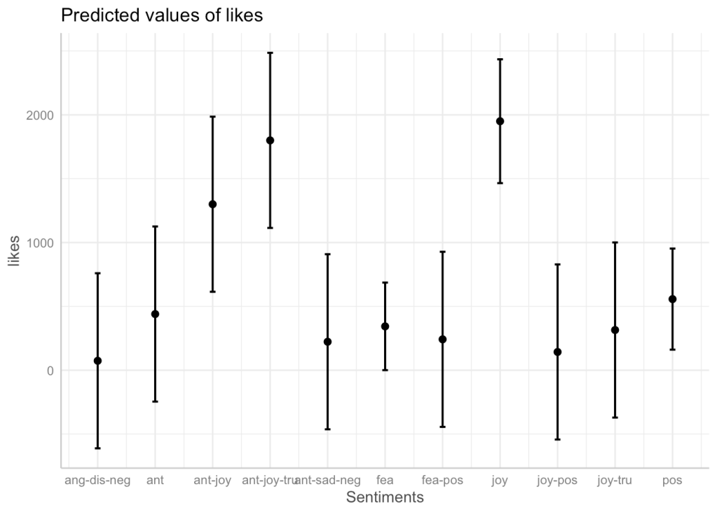
Linear model
We can now finish our model and check out the predicted results and its validity. Before doing so, I have also included a visualization of how the data that we are trying to fit to the model looks like. It is a nice reminder to how our model is most definitely lacking more observations to be taken fully seriously. However, fitting the data is a nice way to study the already existing relationships.
For example, by looking at the figures below, we can see that posts which included joyful words were likely to have more likes, and that even though posts that included fearful words were more likely to receive less likes although it was the most prevalent.
ggplot(lm.data, mapping = aes(y = likes, Sentiments, col = Sentiments, fill =  Sentiments) )+
  geom_boxplot(alpha = .25)+
  ylab('Likes')+theme_bw()+
  theme(legend.position = "none")

ggeffects::ggpredict(lm,
                     c('Sentiments')) %>% plot(
                       jitter = 0
                     )
lm.data %>% head %>% knitr::kable()
| likes | Sentiments | |
|---|---|---|
| 1 | 1300 | ant-joy |
| 2 | 957 | fea |
| 3 | 242 | fea-pos |
| 5 | 143 | joy-pos |
| 6 | 440 | ant |
| 7 | 618 | pos |
stargazer(lm, type = 'html')
| Dependent variable: | |
| likes | |
| Sentimentsant | 366.000 |
| (494.770) | |
| Sentimentsant-joy | 1,226.000** |
| (494.770) | |
| Sentimentsant-joy-tru | 1,726.000** |
| (494.770) | |
| Sentimentsant-sad-neg | 149.000 |
| (494.770) | |
| Sentimentsfea | 269.500 |
| (391.150) | |
| Sentimentsfea-pos | 168.000 |
| (494.770) | |
| Sentimentsjoy | 1,876.000*** |
| (428.483) | |
| Sentimentsjoy-pos | 69.000 |
| (494.770) | |
| Sentimentsjoy-tru | 241.000 |
| (494.770) | |
| Sentimentspos | 483.000 |
| (403.978) | |
| Constant | 74.000 |
| (349.855) | |
| Observations | 17 |
| R2 | 0.900 |
| Adjusted R2 | 0.733 |
| Residual Std. Error | 349.855 (df = 6) |
| F Statistic | 5.400** (df = 10; 6) |
| Note: | p<0.1; p<0.05; p<0.01 |
